Concrete
Regression of concrete compressive strength from the mix and its age, on
the UCI Concrete Compressive Strength dataset (Yeh, 1998). The tutorial
runs four power-basis families side by side, among them a five-input
polyquad, and grows a deep network on a small dataset.
The script is tutorials/concrete/concrete.py, its configuration
tutorials/concrete/concrete.yaml. The configuration's own
checkpoint_dir, ../concrete/checkpoints, is relative to the tutorial
folder, so from the repository root it points outside the repository; the
command above sets it. Each run writes its checkpoints and train.log to a
folder of its own inside it, which the script prints at the end. The script
draws the network with Graphviz, so it needs the viz extra.
Data
1,030 concrete mixes, each described by 8 features: the amounts of cement,
blast furnace slag, fly ash, water, superplasticizer, coarse and fine
aggregate (kg/m³) and the age at testing (days). The target is the
compressive strength in MPa, from 2.3 to 82.6. On its first run, the script
downloads a CSV copy of the dataset and caches it in
tutorials/concrete/data/.
The script takes the log of the age, which the experiment spaces logarithmically from 1 to 365 days. It holds out 20% of the rows for test and splits the rest 4:1 into train and dev: 659, 165 and 206 rows. It standardizes the features and the target on the training rows, and turns the predictions back into MPa before it scores them.
The configuration
| Setting | Value | Why |
|---|---|---|
model.ref_functions |
linear_cov, quadratic, cubic, polyquad with dim: 5 |
pairwise products, squares, cubes and a five-input quadratic compete in every layer |
model.shortcut |
true | every layer can still read the 8 features |
model.nbest_neurons, model.max_neuron_models |
8, 56 | 8 survivors per layer; up to 56 candidates per family, which polyquad with dim: 5 requires (see Power-basis polynomials) |
train.neuron_selection_method |
omp_mixed, threshold 0.2 |
survivors whose outputs differ (see Survivor selection) |
train.ridge_alpha |
0.001 | a small L2 penalty on the coefficients |
train.optimizer |
lbfgs, lr 0.1, min_lr 0.01 |
one batch holds every training row |
train.criterion_minimum_width, train.max_layer_count |
2, 50 | the search stops after two layers without improvement |
model.use_output_projection |
false | the best neuron of the last layer predicts; the out_proj_train block in the file applies once the head is turned on |
Results
Two runs of the configuration as shipped on a CPU gave the same numbers, about 8 minutes each. The search trained 32 layers and kept 30: the dev error fell from 0.1493 at the first layer to 0.0682 at the thirtieth, then stopped improving.
| Test metric | Value |
|---|---|
| RMSE | 5.3731 MPa |
| MAE | 4.0153 MPa |
| R² | 0.8880 |
The model uses all 8 features, and the pruned model scores the same.
The network
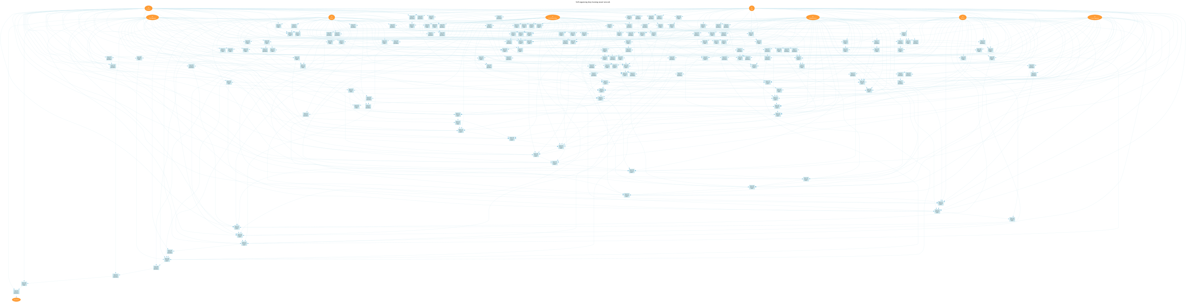
The script draws the trained network into concrete_model.svg and the
pruned one into concrete_pruned_model.svg, next to the script. With 30
layers the drawings are large; open them on their own:
the whole network and
the pruned network.
The copies in the repository come from a different run and show 34
layers; each run of the script draws them anew.

Checked against TorchSONN 0.1.5.