Gaussian RBF

The polynomial families fit a global basis: every term is nonzero almost everywhere. The rbf family fits a local one. Each neuron places \(M\) Gaussian bumps over the space of its inputs and learns the weights of the bumps together with where the bumps sit and how wide they are. Each bump is active only near its own centre and fades away from it, so together they cover the range in overlapping patches:

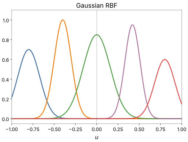
The neuron

The neuron first standardizes each of its inputs with that input's mean and standard deviation, giving \(u\). Bump \(m\), with centre \(c_m\) and width \(s_m\), measures the scaled squared distance

\[ d_m(u) = \frac{\lVert u - c_m \rVert^2}{2 s_m^2} . \]

By default the bump activations are normalized to sum to 1,

\[ \varphi_m(u) = \frac{e^{-d_m(u)}}{\sum_{k=1}^{M} e^{-d_k(u)}} , \]

so every row is a weighted blend of the bumps nearest to it, and rows far from every centre still get a well-defined value. The design row is the \(M\) bump activations followed by the standardized inputs themselves, a linear part:

\[ \big[\ \varphi_1(u), \dots, \varphi_M(u),\ u_1, \dots, u_{\text{dim}}\ \big] \]

That is \(M + \text{dim}\) weights: 18 for a pair with the default 16 centres. The normalized bumps already sum to 1, so no constant column is needed. With normalize: false the plain Gaussians \(e^{-d_m(u)}\) are used and a constant column is added; with linear: false the linear part is dropped.

A network with rbf neurons is not a polynomial (see the Kolmogorov-Gabor polynomial).

Where the bumps start

Before a layer trains, the input pass places every candidate's bumps on a sample of that candidate's inputs from the train split:

• placement: kmeans (default) runs k-means with \(M\) clusters on the sample. The default start, seeding: pca_quantiles, takes the rows at evenly spaced quantiles along the first principal axis of the inputs. It depends on the data only, so the same data gives the same centres under any seed, making runs reproducible regardless of the seed. seeding: kmeans++ draws a k-means++ start from the seeded generator instead. Lloyd iterations then refine the centres (train.rbf_kmeans_iters, 20 by default).
• placement: grid places the bumps on a grid of quantiles of each input, from the 10th to the 90th percentile, \(K\) points per input. \(M\) must then be \(K^{\text{dim}}\), for example 9, 16 or 25 for a pair.

The sample holds up to train.input_sample_rows rows (65,536 by default), drawn uniformly from the split. train.rbf_kmeans_mode chooses what happens next. With sample, k-means runs on the sample alone. With stream, the start is taken on the sample and the centres are then refined by mini-batch k-means over the whole split, train.rbf_kmeans_passes passes (1 by default), one batch at a time. auto, the default, streams when the split has more rows than the sample holds and uses the sample otherwise.

Each bump's starting width is width (1 by default) times its local spacing, the mean distance from its centre to the two nearest other centres.

What the fit learns

The centres and widths are learned together with the weights, but each is held near its start by a smooth bound:

\[ c_m = c^{0}_m + r_m \tanh\!\left(\frac{\lVert \delta_m \rVert}{r_m}\right) \frac{\delta_m}{\lVert \delta_m \rVert}, \qquad s_m = s^{0}_m \exp\!\Big(L \tanh\!\big(\rho_m / L\big)\Big) \]

Here \(c^0_m\) and \(s^0_m\) are the placed start, \(\delta_m\) and \(\rho_m\) the learned parameters (zero at the start), \(r_m\) is center_radius times the bump's local spacing, and \(L = \ln(\text{width\_band})\). A centre moves at most \(r_m\) from where k-means put it, and a width stays between \(1/\text{width\_band}\) and \(\text{width\_band}\) times its start. The bound is smooth, so unlike a hard clamp it keeps a gradient everywhere.

The bound keeps every bump on the data. With center_radius: null the centres move freely; then the optimizer matters, since an unconstrained centre can drift far into empty space and become a dead bump with no data and no gradient. The LBFGS safeguards (max_step, curvature_eps) guard against this; with them on, bounding the centres is a safety net rather than an accuracy trade-off.

With learn_centers: false and learn_widths: false, the bumps stay where they were placed and only the weights are fitted: a fixed-basis RBF.

Options

Option	Default	Meaning
centers	16	bumps per neuron, \(M\); at least 2
dim	2	inputs per neuron
placement	kmeans	kmeans or grid
seeding	pca_quantiles	k-means start: pca_quantiles or kmeans++
width	1.0	starting width, times the local spacing
learn_centers	true	learn the centres
learn_widths	true	learn the widths
center_radius	2.0	how far a centre may move, times the local spacing; null for no bound
width_band	4.0	widths stay within this factor of their start; must exceed 1
normalize	true	normalize the bumps to sum to 1
linear	true	add the standardized inputs to the design row
standardize	true	standardize the inputs before the bumps
activation	identity	output activation

model:
  ref_functions:
    - rbf:
        centers: 8

An RBF neuron carries one weight per bump plus the linear part, so an RBF model tends to have many more parameters than a polynomial one of comparable accuracy. The number of centres trades capacity for size: more bumps fit finer local structure but enlarge the model, and past some point add little on smooth data.

In the log

The input pass logs one line per family when it places the centres: the method, the cluster sizes (and how many clusters are empty), and the median starting width and radius. After selection, the trainer logs how far the survivors' centres moved from their start (in standard deviations), the share of centres at their radius, and where the width scales sit, including the share at the band's edge. A fit that never moves a centre, or pushes everything against its bound, shows up there.

The short name is RBF<M>, with the number of inputs when it is not 2: RBF16, RBF8x3.

The knobs

model.ref_functions with the options above, train.input_sample_rows, train.rbf_kmeans_mode, train.rbf_kmeans_iters and train.rbf_kmeans_passes. See Configuration keys.

Checked against TorchSONN 0.1.5.