California housing: torchsonn against gradient boosting¶

This page is the California housing tutorial's README, kept next to its code in tutorials/california_housing/. Run its commands from the repository root; the network diagrams need the viz extra.

This tutorial fits a self-organizing neural network TorchSONN to the California housing regression task. It then compares the result with gradient-boosted trees on the same features and the same split. This page covers the dataset, the published results, what each of the tutorial's settings is worth, and where it stands against XGBoost.

The dataset¶

California housing comes from Pace & Barry, Sparse Spatial Autoregressions (Statistics & Probability Letters, 1997) [1]. It is built from the 1990 US census. Each of its 20,640 rows is a census block group, described by 8 numeric features:

feature	meaning
MedInc	median income in the block group (tens of thousands of dollars)
HouseAge	median house age
AveRooms, AveBedrms	average rooms / bedrooms per household
Population, AveOccup	population, average household size
Latitude, Longitude	position of the block group

The target is the median house value, in units of $100,000. It is censored at 5.0 ($500k), and 4.8% of the rows sit on that cap. The tutorial loads the StatLib copy through sklearn.datasets.fetch_california_housing.

Kaggle. The dataset did not come from a Kaggle competition. It is older than Kaggle, and Kaggle hosts it in two forms:

The "California Housing Prices" dataset. This is the version from Géron's Hands-On Machine Learning [4]. It has raw room and bedroom totals, a categorical ocean_proximity column and some missing values. It is a dataset page with notebooks, not a competition, so it has no official leaderboard.
Playground Series S3E1, "Regression with a Tabular California Housing Dataset" (January 2023) [5]. This is a real competition, scored by RMSE. Its training and test data were synthetic, generated by a deep model trained on California housing. Its leaderboard numbers therefore don't carry over to the real data, and they are not used here.

Published results¶

There is no single official benchmark. The most careful published numbers come from the Yandex tabular deep learning papers [2] [3]. They tune every model on a validation split and report the test RMSE averaged over 15 seeds, using the original 8 features on their own fixed random split (20% test).

Two papers from other groups use the same protocol and confirm the picture:

T2G-Former [7] reuses that exact split, with 15 seeds.
ExcelFormer [8] draws a random 80/20 split the same way, averaging 5 runs.

All numbers are single models:

model	test RMSE	test MSE (RMSE²)	source
MLP	0.499	0.249	Gorishniy et al. 2023 (TabR) [2]
FT-Transformer	0.459	0.211	Gorishniy et al. 2021 [3]
FT-Transformer (tuned)	0.468	0.219	Chen et al. 2024 (ExcelFormer) [8]
T2G-Former	0.455	0.207	Yan et al. 2023 [7]
XGBoost (tuned)	0.436	0.190	Yan et al. 2023 [7]
XGBoost / CatBoost (tuned)	0.436	0.190	Chen et al. 2024 (ExcelFormer) [8]
LightGBM (tuned)	0.434	0.188	TabR paper [2]
XGBoost (tuned)	0.432	0.187	TabR paper [2]
ExcelFormer (mix-tuned)	0.432	0.186	Chen et al. 2024 (ExcelFormer) [8]
CatBoost (tuned)	0.426	0.181	TabR paper [2]
TabR-S	0.403	0.162	TabR paper [2]
TabR (best single model)	0.400	0.160	TabR paper [2]

Two points matter for the comparison below:

On the raw features, tuned gradient boosting lands at 0.426–0.436 RMSE (MSE ≈ 0.18–0.19) across three groups' papers. Transformer-style networks land at 0.455–0.468.
Only two models beat the trees on this protocol: ExcelFormer (0.432), narrowly, and TabR (0.400).
The best published single model, TabR [2], gets its edge by retrieval: it looks up the target values of the most similar training rows. The tutorial's kNN price feature does the same thing for location (see below).

These numbers come from a different split and a different feature set from the tutorial's, so they set the scale, not a like-for-like target. The fair comparison is the tree models run on the tutorial's own data, in the last section.

The tutorial's setup¶

Split. A random 20% of the rows is held out as the test set (4,128 rows, fixed for every run). The rest is split 3:1 into train (12,384 rows), which fits the neurons, and dev (4,128 rows), which selects them.
Features (tutorial.feature_engineering). There are 16 inputs:
logs of the skewed columns;
log bedrooms-per-room and log rooms-per-person;
coordinates rotated 45°;
log distance to Los Angeles, San Francisco, San Diego and San Jose;
the mean log price of the 20 nearest training blocks. This is leave-one-out on the training rows, so it doesn't leak the target.
Target and loss. The model fits the raw price. The loss treats rows at the $500k cap as censored, and predictions are clipped to the training range.
Metrics. Test MSE and MAE on the 4,128 held-out rows, in ($100k)² and $100k.
Candidate early stop. The results below stop each candidate's fit on its training loss, train.early_stop_source=train on the command line, which the config files leave at dev. With it, the Legendre config's seed-10 run keeps 6 layers; without it, the search stops after 4 layers at a test MSE of about 0.187.

Running it¶

From the repo root, with one of the two configs the results below come from and the candidate early stop they use:

python -m tutorials.california_housing.california_housing --config-name california_housing_legendre_finetune \
    train.early_stop_source=train train.checkpoint_dir=checkpoints/california_legendre
python -m tutorials.california_housing.california_housing --config-name california_housing_rbf \
    train.early_stop_source=train train.checkpoint_dir=checkpoints/california_rbf

Both configs set train.checkpoint_dir relative to the tutorial folder, which from the repo root points outside it, so the commands set it. Each run writes its checkpoints, train.log and network diagrams to a folder of its own inside it, which the script logs; the diagrams need the viz extra. Both configs run on the CPU as shipped, and train.device=cuda moves a run to a GPU: the Legendre command took 46 s on an RTX 5080 and scored a test MSE of 0.1843.

Tutorial settings¶

The tutorial section of the configuration holds the script's own settings, read by tutorial_params() in california_housing.py. A key the script does not know stops the run with KeyError.

Key	Default	Meaning
`tutorial.test_size`	0.2	Fraction of the rows held out as the test set.
`tutorial.dev_split`	`sqMode4_1`	How the remaining rows split into train and dev, a `SequenceTypeSet` name; `sqMode4_1` sends every 4th row to dev.
`tutorial.val_split`	0.0	Fraction of the training rows set aside as a validation split; 0 for none.
`tutorial.n_ensemble`	1	Number of models to train, each with its own seed and, after the first, its own shuffle of the non-test rows; the script reports each and the mean of their predictions.
`tutorial.z_clip`	5.0	Standardized features are clipped to ±this value.
`tutorial.feature_engineering`	false	Master switch for the two feature groups below; off, the model sees the eight raw columns. Every config in the folder turns it on.
`tutorial.log_features`	true	Log-transform the skewed features and add the bedrooms-per-room and rooms-per-person ratios.
`tutorial.location_features`	true	Add the rotated coordinates, the log distances to four cities and the kNN price feature.
`tutorial.knn_price_k`	20	Neighbours averaged by the kNN price feature.
`tutorial.log_target`	false	Fit the log of the price instead of the price.
`tutorial.clip_predictions`	true	Clip predictions to the range of the training targets.
`tutorial.censor_cap`	true	Treat targets at the $500k cap as censored in the training loss (`train.censor_target_at`).

What each setting is worth¶

All numbers are single-model test results, as recorded in the config headers [6]. Each row adds one change to the row above it.

step	test MSE	test MAE
Legendre baseline (gmdhpy-style, raw features, 50/50 split)	0.3484	0.4184
+ linear head over the survivors, end-to-end fine-tune, prediction clip	0.3002	0.3758
+ log features, log target	0.3013	0.3626
+ location features (rotated coordinates, city distances, kNN price)	0.2605	0.3307
60/20/20 split (train 12,384 rows) ¹	0.2160	0.2975
per-layer fine-tune off, 16 survivors	0.1972	0.2786
decorrelated survivor selection (`omp_mixed`)	0.1946	0.2731
feature audit (log MedInc, bedrooms-per-room ratio)	0.1920	0.2740
censored loss at the $500k cap	0.1912	0.2719
raw instead of log target (MSE favours the mean)	0.1877	0.2791
24 survivors (mean of seeds 10–13)	0.1852 ± 0.0008	0.2775

¹ This step changes the test set. On the same 4,128 test rows, the model from the row above scores 0.2650, so about 0.05 of this step's gain comes from the extra training data.

The kNN price feature carries most of the location gain. Without it, the first layer's error is 0.42; with it, 0.185.

Experiments with different configs¶

Several dozen runs, each followed by seed repeats, tested the remaining settings:

neuron families and polynomial degree;
candidate caps and survivor count;
the survivor selection rule;
the stop rules;
the end-to-end learning rate.

Seed noise. A fixed seed repeats to 0.0004. Changing the seed changes which candidate pairs are sampled, and that moves the test MSE by up to 0.009. A single-run difference under about 0.005 is therefore not a finding.

Seed-repeated results (seeds 10–13, test MSE / MAE):

configuration	mean MSE ± sd	mean MAE
Legendre-3, 16 survivors	0.1890 ± 0.0031	0.2793
RBF-8, 16 survivors	0.1909 ± 0.0016	0.2793
Legendre + RBF-8, 16 survivors	0.1898 ± 0.0022	0.2797
Legendre-3, 32 survivors	0.1851 ± 0.0023	0.2764
Legendre + RBF-8, cap 500, 32 survivors	0.1860 ± 0.0021	0.2753
Legendre degree 5	0.1868 ± 0.0027	0.2788
`linear_cov` instead of Legendre, 24 survivors	0.1990 ± 0.0021	0.2924
`quadratic` instead of Legendre, 24 survivors	0.2027 ± 0.0054	0.2941
Legendre-3, 24 survivors (as shipped)	0.1852 ± 0.0008	0.2775
RBF-8, 24 survivors (as shipped)	0.1853 ± 0.0014	0.2772

What the experiments found:

Survivor selection is the strongest lever. Plain and omp selection cost 0.009–0.015.
A wider survivor pool is the one robust gain. 32 survivors beat 16 on every seed, and 24 survivors gave the same mean with the smallest spread. 48 survivors lose.
Everything else is inside the noise:
polynomial degree 4 or 5;
Chebyshev instead of Legendre;
adding a linear neuron family next to Legendre;
RBF centre counts of 4 to 16;
grid or unbounded RBF centres;
the stop-rule variants.
Some changes are clear losses:
the power-basis families instead of Legendre: linear_cov (+0.014) and quadratic (+0.018). quadratic has more terms but is no better and is the least stable across seeds. Its searches stop after 4–5 layers, against 7–10 for Legendre. Unlike Legendre, these neurons do not squash their inputs, and raw powers of heavy-tailed features are poorly conditioned;
dropping the head (+0.009);
the per-layer fine-tune;
a strong ridge on RBF weights;
a fixed RBF basis.

Legendre-3 and RBF-8 tie at 0.185.

Against gradient boosting, same data¶

The tree models and the MLP below are fitted on the tutorial's exact 16 features, the same train/dev/test rows and the same prediction clip. Each model is reported as the mean ± standard deviation over several seeds.

"Learned parameters" counts everything the model learned:

Trees: each split counts as 2 (the feature it splits on and the threshold), and each leaf value counts as 1.
MLP: every weight and bias. 16 inputs → 64 hidden units → 1 output gives 16·64 + 64 + 64 + 1 = 1,153.
SONN: each Legendre neuron has 8 coefficients (a degree-3 polynomial of two inputs). Each RBF-8 neuron has 66: 18 weights, 16 centre coordinates and 16 widths. The 24→1 head has 25 weights. SONN models are counted after pruning to the neurons that reach the output.

The parameter column shows the smallest model among the seeds.

model	seeds	mean test MSE ± sd	test RMSE	mean test MAE	learned parameters
sklearn HistGradientBoosting (lr 0.05, 31 leaves)	0–4	0.1697 ± 0.0015	0.412	0.2649	22,477 ¹
XGBoost (hist, depth 6, lr 0.05, early stop on dev)	0–4	0.1719 ± 0 ²	0.415	0.2632	52,257 ²
torchsonn Legendre-3, 24 survivors	10–13	0.1852 ± 0.0008	0.430	0.2775	801 ³
torchsonn RBF-8, 24 survivors	10–13	0.1853 ± 0.0014	0.430	0.2772	6,485 ⁴
MLP, one hidden layer of 64 units (SiLU)	0–4	0.1905 ± 0.0012	0.436	0.2871	1,153 ⁵

¹ The seed changes HistGradientBoosting's internal early-stopping split. The five models have 247–459 trees and 22,477–41,769 parameters.

² With no row or column subsampling, XGBoost is deterministic. Every seed gives the same 339 trees and the same result.

³ The pruned models have 801, 1,009, 1,001 and 801 parameters (seeds 10–13). The 801-parameter seed-10 model is also the most accurate of the four: test MSE 0.1841.

⁴ The pruned models have 8,185, 6,485, 9,953 and 8,049 parameters (seeds 10–13). The 6,485-parameter seed-11 model is also the most accurate: test MSE 0.1830. RBF-8 matches Legendre-3 on accuracy, but it saves far fewer parameters relative to the trees.

⁵ Wider single hidden layers barely help: 256 units give 0.1891 ± 0.0013 (4,609 parameters) and 1,024 units give 0.1894 ± 0.0010 (18,433 parameters). 16 units give 0.1918 ± 0.0032 (289 parameters).

Neither tree model nor the MLP was tuned beyond these settings.

Reproducing the tree models. The script below builds the tutorial's features and split with the tutorial's own functions, then fits both models. Run it from the repo root (pip install xgboost if needed). It prints the per-seed numbers behind the table.

Show the script

import numpy as np
import xgboost as xgb
from omegaconf import OmegaConf
from sklearn.datasets import fetch_california_housing
from sklearn.ensemble import HistGradientBoostingRegressor
from sklearn.metrics import mean_absolute_error, mean_squared_error
from sklearn.model_selection import train_test_split

from torchsonn.data.preprocessing import split_dataset
from tutorials.california_housing import california_housing as ch

# The tutorial's features and split: 16 inputs, 20% test, train/dev 3:1.
p = ch.tutorial_params(OmegaConf.create({"tutorial": {"feature_engineering": True}}))
data = fetch_california_housing()
X, names = ch.engineer_features(data.data.astype(np.float32), list(data.feature_names), p)
y = data.target.astype(np.float32)
X_rest, X_test, y_rest, y_test = train_test_split(X, y, test_size=p.test_size, random_state=42)
X_train, y_train, X_dev, y_dev = split_dataset(X_rest, y_rest, p.dev_split)

# kNN price feature, fitted on the training rows only.
ll = [names.index("Latitude"), names.index("Longitude")]
knn_train, knn_dev, knn_test = ch.knn_price_feature(
    X_train[:, ll], np.log(y_train), [X_dev[:, ll], X_test[:, ll]], p.knn_price_k)
X_train = np.column_stack([X_train, knn_train])
X_dev = np.column_stack([X_dev, knn_dev])
X_test = np.column_stack([X_test, knn_test])


def report(name, y_pred):
    y_pred = np.clip(y_pred, y_train.min(), y_train.max())  # same clip as the tutorial
    print(f"{name}: test MSE {mean_squared_error(y_test, y_pred):.4f}  "
          f"MAE {mean_absolute_error(y_test, y_pred):.4f}")


for seed in range(5):
    hgb = HistGradientBoostingRegressor(
        learning_rate=0.05, max_leaf_nodes=31, l2_regularization=1.0, min_samples_leaf=20,
        max_iter=5000, early_stopping=True, validation_fraction=0.15, n_iter_no_change=50,
        random_state=seed)
    hgb.fit(X_train, y_train)
    report(f"HistGradientBoosting, seed {seed}", hgb.predict(X_test))

booster = xgb.XGBRegressor(
    n_estimators=5000, learning_rate=0.05, max_depth=6, tree_method="hist",
    early_stopping_rounds=50, random_state=0)
booster.fit(X_train, y_train, eval_set=[(X_dev, y_dev)], verbose=False)
report("XGBoost", booster.predict(X_test, iteration_range=(0, booster.best_iteration + 1)))

Reproducing the MLP. The script below builds the same features and split, standardizes the inputs on the training rows and fits a single-hidden-layer MLP with PyTorch. It trains with AdamW and plain MSE, halves the learning rate when the dev loss stalls, and stops early on dev, keeping the best epoch. Run it from the repo root. It prints the per-seed numbers behind the table (the numbers above came from a CUDA run).

Show the script

import numpy as np
import torch
from omegaconf import OmegaConf
from sklearn.datasets import fetch_california_housing
from sklearn.metrics import mean_absolute_error, mean_squared_error
from sklearn.model_selection import train_test_split

from torchsonn.data.preprocessing import split_dataset
from tutorials.california_housing import california_housing as ch

# The tutorial's features and split: 16 inputs, 20% test, train/dev 3:1.
p = ch.tutorial_params(OmegaConf.create({"tutorial": {"feature_engineering": True}}))
data = fetch_california_housing()
X, names = ch.engineer_features(data.data.astype(np.float32), list(data.feature_names), p)
y = data.target.astype(np.float32)
X_rest, X_test, y_rest, y_test = train_test_split(X, y, test_size=p.test_size, random_state=42)
X_train, y_train, X_dev, y_dev = split_dataset(X_rest, y_rest, p.dev_split)

# kNN price feature, fitted on the training rows only.
ll = [names.index("Latitude"), names.index("Longitude")]
knn_train, knn_dev, knn_test = ch.knn_price_feature(
    X_train[:, ll], np.log(y_train), [X_dev[:, ll], X_test[:, ll]], p.knn_price_k)
X_train = np.column_stack([X_train, knn_train])
X_dev = np.column_stack([X_dev, knn_dev])
X_test = np.column_stack([X_test, knn_test])

# Standardize the inputs on the training rows.
device = "cuda" if torch.cuda.is_available() else "cpu"
mu, sd = X_train.mean(0), X_train.std(0) + 1e-8
Xtr, Xdv, Xte = (torch.tensor((a - mu) / sd, device=device) for a in (X_train, X_dev, X_test))
ytr, ydv = torch.tensor(y_train, device=device), torch.tensor(y_dev, device=device)


def report(name, y_pred):
    y_pred = np.clip(y_pred, y_train.min(), y_train.max())  # same clip as the tutorial
    print(f"{name}: test MSE {mean_squared_error(y_test, y_pred):.4f}  "
          f"MAE {mean_absolute_error(y_test, y_pred):.4f}")


def fit_mlp(hidden, seed, epochs=2000, patience=100, batch_size=256):
    torch.manual_seed(seed)
    model = torch.nn.Sequential(
        torch.nn.Linear(Xtr.shape[1], hidden), torch.nn.SiLU(), torch.nn.Linear(hidden, 1)).to(device)
    opt = torch.optim.AdamW(model.parameters(), lr=3e-3, weight_decay=1e-4)
    sched = torch.optim.lr_scheduler.ReduceLROnPlateau(opt, factor=0.5, patience=30)
    best, best_state, bad = float("inf"), None, 0
    for _ in range(epochs):
        model.train()
        perm = torch.randperm(len(Xtr), device=device)
        for i in range(0, len(Xtr), batch_size):
            idx = perm[i:i + batch_size]
            loss = ((model(Xtr[idx]).squeeze(1) - ytr[idx]) ** 2).mean()
            opt.zero_grad()
            loss.backward()
            opt.step()
        model.eval()
        with torch.no_grad():
            dev_mse = ((model(Xdv).squeeze(1) - ydv) ** 2).mean().item()
        sched.step(dev_mse)
        if dev_mse < best - 1e-6:  # early stop on dev, keep the best epoch
            best, bad = dev_mse, 0
            best_state = {k: v.clone() for k, v in model.state_dict().items()}
        else:
            bad += 1
            if bad > patience:
                break
    model.load_state_dict(best_state)
    with torch.no_grad():
        return model(Xte).squeeze(1).cpu().numpy()


for seed in range(5):
    report(f"MLP (64 hidden units), seed {seed}", fit_mlp(64, seed))

The models¶

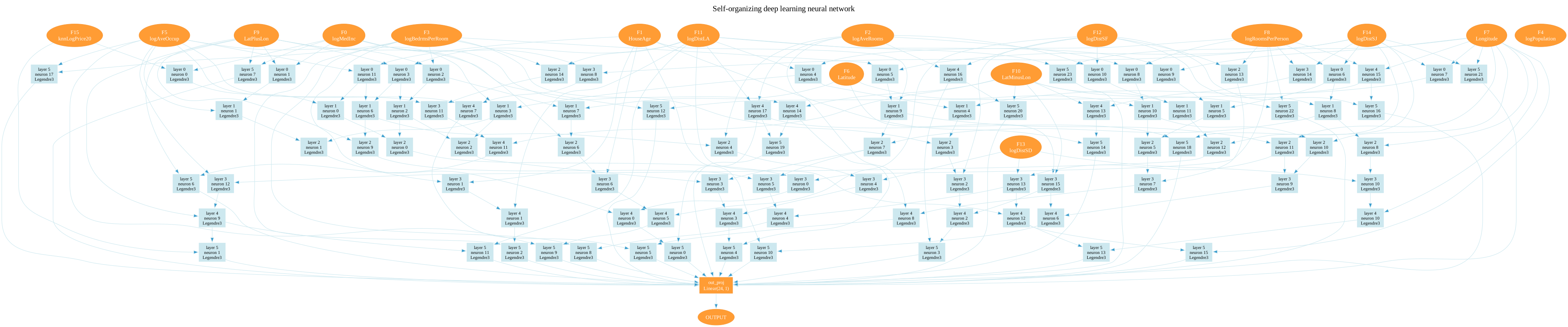
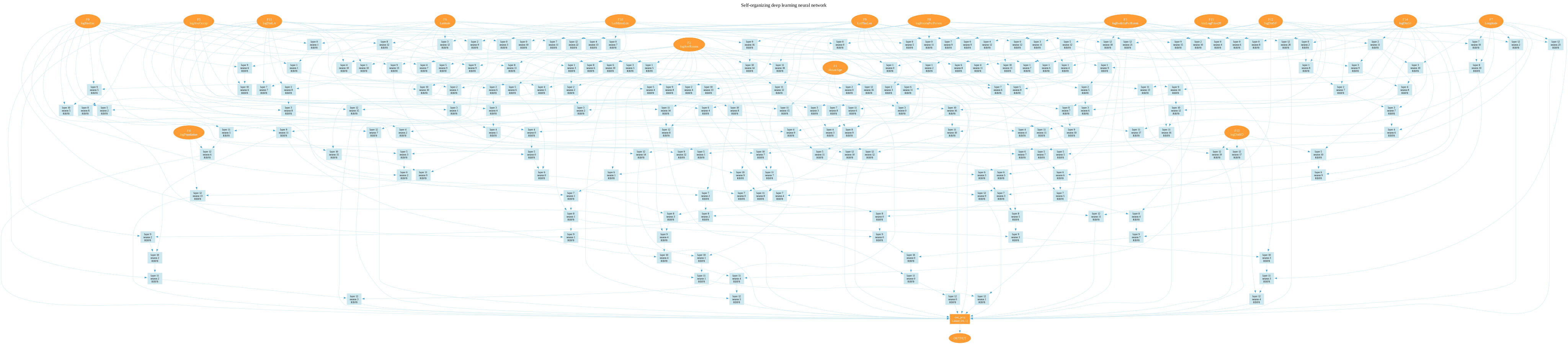
These are the pruned networks of two of the seed runs above, cut down to the neurons that reach the output. Each box is a neuron, and its two incoming edges are the inputs its polynomial reads. The final linear head combines the 24 survivors of the last layer.

Legendre-3, best model (seed 10, test MSE 0.1841): 6 layers and 801 learned parameters after pruning. It uses 15 of the 16 inputs; only logPopulation is left out. The unpruned network has 1,177 parameters: unpruned_legendre_best.svg.

Pruned Legendre-3 network (click to expand; click the image for full size)

RBF-8, smallest model (seed 11, test MSE 0.1830, also the most accurate RBF-8 seed): 13 layers and 6,485 learned parameters after pruning, using all 16 inputs. The unpruned network has 10,633 parameters: unpruned_rbf8_smallest.svg.

Pruned RBF-8 network (click to expand; click the image for full size)

Summary¶

torchsonn does not outperform gradient boosting on California housing. On identical features and splits:

the best tree model reaches a mean test MSE of 0.170;
torchsonn reaches 0.185;
a single-hidden-layer MLP reaches 0.191.

That is a gap of 0.015 MSE, or about 0.018 RMSE (0.412 vs 0.430). No seed of either torchsonn model reaches the trees' worst seed.

The settings in What each setting is worth take the tutorial from 0.348, for the plain Legendre setup, to within 9% of the trees. Its 0.430 RMSE is on a par with the tuned XGBoost and LightGBM numbers published for this dataset (0.432 and 0.434, on their split and features) [2].

The Legendre model gets there with about 30–65× fewer learned parameters: 801 polynomial coefficients after pruning, against 22,000 to 52,000 split thresholds and leaf values. The RBF-8 family reaches the same accuracy, but with 6,500 parameters it is only 3–8× smaller than the trees, so the saving belongs to the Legendre model.

The result is also interpretable and trainable in ways the tree ensembles are not:

every neuron is an explicit degree-3 polynomial of two named inputs;
the network can be rendered as a graph (see The models);
the script reports which input features the model actually uses;
the whole network is differentiable, so it can be fine-tuned by gradient descent on new data. A tree ensemble's splits are fixed once grown; it can only be extended with more trees or retrained.

References¶

R. K. Pace, R. Barry, Sparse Spatial Autoregressions, Statistics & Probability Letters 33 (1997) 291–297.
Y. Gorishniy et al., TabR: Tabular Deep Learning Meets Nearest Neighbors (2023): https://arxiv.org/abs/2307.14338
Y. Gorishniy et al., Revisiting Deep Learning Models for Tabular Data (2021): https://arxiv.org/abs/2106.11959
A. Géron, Hands-On Machine Learning with Scikit-Learn and TensorFlow (O'Reilly, 2017); its copy of the data on Kaggle: https://www.kaggle.com/datasets/camnugent/california-housing-prices
Kaggle Playground Series S3E1, Regression with a Tabular California Housing Dataset: https://www.kaggle.com/competitions/playground-series-s3e1
The results tables in the headers of california_housing_legendre_finetune.yaml and california_housing_rbf.yaml.
J. Yan et al., T2G-Former: Organizing Tabular Features into Relation Graphs Promotes Heterogeneous Feature Interaction (AAAI 2023): https://arxiv.org/abs/2211.16887
J. Chen et al., ExcelFormer: A Neural Network Surpassing GBDTs on Tabular Data (KDD 2024): https://arxiv.org/abs/2301.02819