Combined Cycle Power Plant (CCPP) regression¶
This page is the CCPP tutorial's README, kept next to its code in
tutorials/ccpp/. Run its commands from the repository root; the network
diagrams need the viz extra.
A TorchSONN tutorial that reproduces the canonical UCI Combined Cycle Power
Plant benchmark: predict a plant's net hourly electrical output PE (MW) from
four hourly-average ambient measurements, and evaluate with the 5×2
cross-validation protocol that every published CCPP result is measured
against.
The plant runs a gas turbine and a steam turbine in tandem; four ambient variables set the operating point, and the model predicts the net output:
| Feature | Meaning | Unit | Effect on output |
|---|---|---|---|
AT |
Ambient Temperature | °C | strong negative driver (r ≈ −0.95) |
V |
Exhaust Vacuum | cm Hg | strong negative driver (r ≈ −0.87) |
AP |
Ambient Pressure | millibar | mild positive driver (r ≈ +0.52) |
RH |
Relative Humidity | % | mild positive driver (r ≈ +0.39) |
PE |
Net electrical output (target) | MW | range 420–496 MW |
The relationship is predominantly linear — a plain linear fit already reaches
R² ≈ 0.93 — so this is a clean demonstration of SONN discovering that
structure with a linear_cov neuron and then squeezing out the residual
curvature and interactions (the AT×V collinearity, humidity's
temperature-dependent effect) with quadratic and a full four-input polyquad
neuron. Because TorchSONN is itself a self-organizing polynomial network, it
lands squarely in the model class that has been shown to be state-of-the-art
competitive on this dataset (see Comparison).
- Dataset: https://archive.ics.uci.edu/dataset/294/combined+cycle+power+plant
(9568 samples, 4 features; the tutorial auto-downloads a byte-identical CSV
mirror and caches it under
data/ccpp.csv). - Entry point:
ccpp.py - Configs:
ccpp.yaml(light, default) ·ccpp_heavy.yaml(heavy) ·ccpp_legendre.yaml·ccpp_legendre_heavy.yaml·ccpp_legendre_poly.yaml·ccpp_legendre_poly_heavy.yaml(Legendre-basis variants) ·ccpp_mix.yaml(monomial + Legendre families side by side) ·ccpp_legendre_finetune.yaml·ccpp_legendre_poly_finetune.yaml·ccpp_legendre_heavy_finetune.yaml·ccpp_legendre_poly_heavy_finetune.yaml(fine-tuned variants — the strongest results here)
Why 5×2 cross-validation?¶
A single train/test split yields one number whose third decimal is noise — a different random split can swing R² by ±0.005. Tüfekci & Kaya (2014), the paper every CCPP result is measured against, use 5×2 CV: shuffle the data and cut it in half, train on half A / test on half B, then swap (train B / test A) — that is one "2-fold" repeat; do it for five independent shuffles → 5 × 2 = 10 train/test measurements, and report the mean ± standard deviation. The spread across the 10 tells you how stable the number actually is. The tutorial trains the model from scratch on all 10 folds and reports mean ± std of RMSE / MAE / R².
Running it¶
From the repo root:
# Default (light) config — small survivor pool / candidate cap, CPU.
python -m tutorials.ccpp.ccpp

# Heavy config — larger pools + cubic/poly5/poly10 neurons, CUDA.
python -m tutorials.ccpp.ccpp --config-name=ccpp_heavy

# Best accuracy per minute — Legendre + the fine-tuning stack, CPU (~51 min).
python -m tutorials.ccpp.ccpp --config-name=ccpp_legendre_poly_finetune
Every config key is overridable on the command line via Hydra:
python -m tutorials.ccpp.ccpp train.device=cpu
python -m tutorials.ccpp.ccpp model.ref_functions='[linear_cov]' train.max_layer_count=3
python -m tutorials.ccpp.ccpp -m train.ridge_alpha=0.001,0.01,0.05   # multirun sweep
Each fold has a folder checkpoints/fold_NN/, and every run of that fold gets
a time-stamped folder inside it, fold_NN/YYYY-MM-DD-HH-MM-SS/, with the run's
checkpoints and its train.log. The whole cross-validation run is logged to
checkpoints/cv_YYYY-MM-DD-HH-MM-SS.log, which ends with the run folder of
every fold and the summary. After the CV
loop, the discovered network from the final fold is rendered to
ccpp_model.svg (the whole layer stack) and
ccpp_pruned_model.svg (the same network reduced to
the neurons that actually reach the output). Rendering needs the [viz] extra
(pip install "torchsonn[viz]" + system Graphviz).
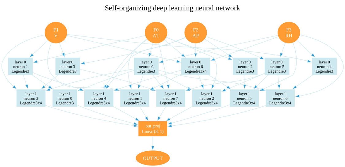
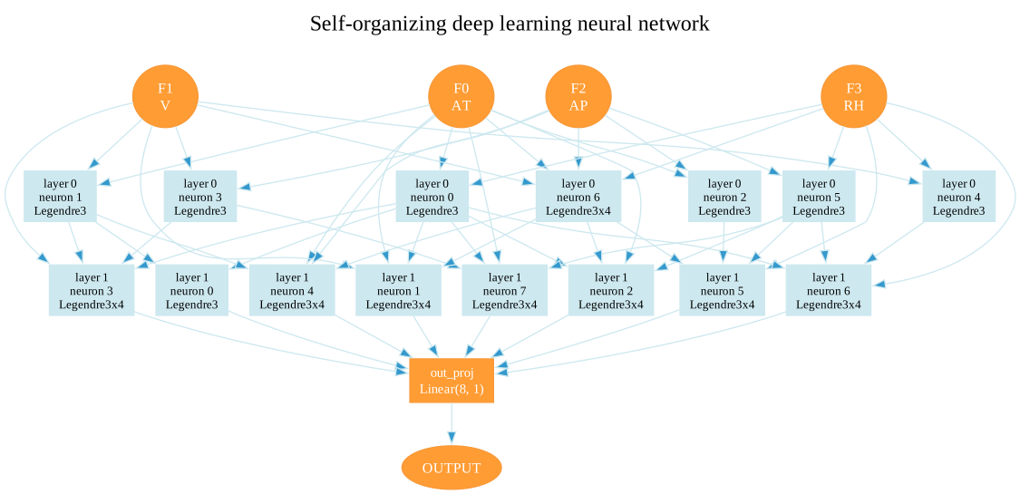
How much the second one reduces depends on whether the config has an output head, and the difference is worth understanding before reading either diagram:
- Without a head (
ccpp.yamland every other non-fine-tuned config) the prediction is one neuron's output, so pruning collapses the network to the single best-error path — a readable "discovered formula", which is the diagram's main purpose. - With a head (the
*_finetuneconfigs, which setuse_output_projection: True) the prediction is a fitted linear combination ofnum_out_neuronscolumns, so all of them reach the output and there is usually nothing to prune. The two SVGs then come out identical, and the model is not reducible to a single formula. Both diagrams draw the head as anout_projnode with an edge from every column it reads.
The committed SVGs are whatever the last run produced, so they may be from
either kind of config; the out_proj node tells you which.
The two base configs¶
These two are the reference points; the Legendre variants below are derived from them, and All configs at a glance puts every config in one table.
| Setting | ccpp.yaml (default) |
ccpp_heavy.yaml |
|---|---|---|
| Reference functions | linear_cov, quadratic, polyquad(dim 4) |
+ cubic, polyquad(dim 5), polyquad(dim 10) |
nbest_neurons (survivors/layer) |
8 | 120 |
max_neuron_models (candidates/family) |
60 | 1200 |
| Device | CPU | CUDA |
| Wall-clock (hardware) | ≈ 19 min | ≈ 11.3 h |
The light config is deliberately cheap so the full 10-fold run is tractable; the heavy config is the larger search used while exploring the model. As the results below show, the heavy config buys only ~0.08 MW of MAE for ~36× the compute — and both are beaten by a light-pool Legendre config with fine-tuning in under an hour on a CPU.
Hardware¶
Every wall-clock figure in this README is hardware-dependent and quoted only to illustrate the cost/accuracy trade-off. All runs were measured on the same machine:
- CPU (
device: cpuconfigs) — 12th-gen Intel Core i9-12900 (16 cores: 8 P + 8 E); ≈ 19 min for the default config. - GPU (
device: cudaconfigs) — NVIDIA GeForce RTX 5080; ≈ 11.3 h for the heavy config.
Results¶
Each block below is the final summary printed by ccpp.py (the ==== section
at the end of the run's log, cited under each heading), reproduced verbatim.
All configs at a glance¶
Sorted by MAE, the canonical CCPP metric. Wall-clock is hardware-dependent —
see Hardware — and quoted only for the cost/accuracy trade-off.
All ccpp_legendre* configs run squash: True with the default sigma
method; the per-config sections below compare each with a squash: False
run of the same config. ccpp_mix.yaml is the exception and stays unsquashed.
The *_finetune rows add the fine-tuning stack
on top of the config they are named after, and nothing else.
All rows were measured with torchsonn 0.1.1, whose regression criterion
divides by Σy², the form train.error_normalization: energy selects. The
configs use the default, variance (Σ(y-ȳ)²), so a rerun can differ
slightly from these rows.
| Config | Families | Pools (nbest/max) | Device | Wall-clock | MAE (MW) | RMSE (MW) | R² |
|---|---|---|---|---|---|---|---|
ccpp_legendre_poly_heavy_finetune.yaml |
linear_cov + Legendre pair & dim 4/6 |
60/600 | CUDA | ≈ 14.7 h | 3.1284 ± 0.0485 | 4.0943 ± 0.0662 | 0.9424 ± 0.0017 |
ccpp_legendre_heavy_finetune.yaml |
Legendre pair (deg 3 + deg 2) | 60/600 | CUDA | ≈ 2.5 h | 3.1408 ± 0.0620 | 4.0890 ± 0.0688 | 0.9426 ± 0.0017 |
ccpp_legendre_poly_finetune.yaml |
Legendre pair + dim 4 | 8/60 | CPU | ≈ 51 min | 3.1495 ± 0.0696 | 4.0940 ± 0.0773 | 0.9424 ± 0.0021 |
ccpp_legendre_finetune.yaml |
Legendre pair (deg 3) | 8/60 | CPU | ≈ 65 min | 3.1748 ± 0.0520 | 4.1152 ± 0.0539 | 0.9418 ± 0.0014 |
ccpp_heavy.yaml |
monomial, + cubic / polyquad(5, 10) |
120/1200 | CUDA | ≈ 11.3 h | 3.2599 ± 0.0356 | 4.1815 ± 0.0486 | 0.9400 ± 0.0010 |
ccpp_legendre_poly_heavy.yaml |
linear_cov + Legendre pair & dim 4/6 |
60/600 | CUDA | ≈ 8.8 h | 3.2777 ± 0.0200 | 4.2111 ± 0.0395 | 0.9391 ± 0.0008 |
ccpp_legendre_poly.yaml |
Legendre pair + dim 4 | 8/60 | CPU | ≈ 25 min | 3.2782 ± 0.0135 | 4.2174 ± 0.0339 | 0.9389 ± 0.0007 |
ccpp_legendre_heavy.yaml |
Legendre pair (deg 3 + deg 2) | 60/600 | CUDA | ≈ 1.4 h | 3.3035 ± 0.0162 | 4.2339 ± 0.0350 | 0.9384 ± 0.0008 |
ccpp_mix.yaml |
monomial + Legendre pair (deg 2 + 3) | 8/60 | CPU | ≈ 56 min | 3.3050 ± 0.0263 | 4.2251 ± 0.0470 | 0.9387 ± 0.0010 |
ccpp_legendre.yaml |
Legendre pair (deg 3) | 8/60 | CPU | ≈ 12 min | 3.3084 ± 0.0147 | 4.2518 ± 0.0322 | 0.9379 ± 0.0007 |
ccpp.yaml (default) |
linear_cov, quadratic, polyquad(4) |
8/60 | CPU | ≈ 19 min | 3.3423 ± 0.0256 | 4.2593 ± 0.0511 | 0.9377 ± 0.0012 |
The fine-tuned configs sweep the top of the table on all three metrics, and by a wide margin: every one of them beats the 11.3 h heavy monomial search, the best of the searches without it, and the best of them does so by 0.13 MW of MAE. Two of the four run on a CPU in under an hour.
They are also barely distinguishable from one another. The four span 3.1284–3.1748 MAE — a 0.046 MW range against fold spreads of ±0.05–0.07 — while their cost spans 51 minutes of CPU to 14.7 hours of GPU, a factor of ~17. The 14.7 h poly-heavy run takes the best MAE by 0.021 MW over the 51-minute poly-light one, which is well inside the noise, and does not take the best RMSE or R². Once the fine-tune is on, the search budget stops mattering.
Among the searches themselves the picture is the one the sections below
develop: ccpp_legendre_poly.yaml matches the 8.8 h poly-heavy GPU run
(3.2782 ± 0.0135 vs 3.2777 ± 0.0200) on light pools and a CPU in ~25 minutes, so
pool width buys almost nothing on this dataset while neuron arity does. The
Legendre configs also carry the tightest spreads, a direct consequence of the
squash — though note the fine-tune trades some of that back (±0.06–0.07 against
±0.01–0.02), which the fine-tuning section discusses.
Default — ccpp.yaml¶
run checkpoints/2026-07-22-19-59-00/train.log — light config, CPU
==================================================================
5×2 cross-validation summary — 10 train/test measurements
==================================================================
repeat   fold   RMSE(MW)    MAE(MW)        R²
     1    A→B     4.2246     3.3675    0.9390
     1    B→A     4.3290     3.3655    0.9353
     2    A→B     4.2797     3.3309    0.9374
     2    B→A     4.2232     3.3129    0.9385
     3    A→B     4.2330     3.3369    0.9385
     3    B→A     4.2966     3.3621    0.9366
     4    A→B     4.2662     3.3432    0.9380
     4    B→A     4.2445     3.3497    0.9376
     5    A→B     4.1670     3.2897    0.9393
     5    B→A     4.3290     3.3643    0.9367
------------------------------------------------------------------
  RMSE = 4.2593 ± 0.0511 MW
  MAE  = 3.3423 ± 0.0256 MW
  R²   = 0.9377 ± 0.0012
Heavy — ccpp_heavy.yaml¶
run checkpoints/2026-07-22-23-11-00/train.log — heavy config, CUDA
==================================================================
5×2 cross-validation summary — 10 train/test measurements
==================================================================
repeat   fold   RMSE(MW)    MAE(MW)        R²
     1    A→B     4.2135     3.3002    0.9394
     1    B→A     4.1894     3.2276    0.9394
     2    A→B     4.1846     3.2324    0.9401
     2    B→A     4.1349     3.2461    0.9411
     3    A→B     4.1307     3.2188    0.9414
     3    B→A     4.2051     3.2855    0.9393
     4    A→B     4.2126     3.2992    0.9396
     4    B→A     4.1656     3.2581    0.9399
     5    A→B     4.1070     3.2219    0.9411
     5    B→A     4.2713     3.3092    0.9384
------------------------------------------------------------------
  RMSE = 4.1815 ± 0.0486 MW
  MAE  = 3.2599 ± 0.0356 MW
  R²   = 0.9400 ± 0.0010
The ccpp_legendre.yaml and ccpp_legendre_heavy.yaml variants replace the
default's monomial neurons (linear_cov / quadratic / polyquad) with a
Legendre orthogonal-polynomial basis over each input pair — a
better-conditioned stand-in for the raw cubic terms, since the Legendre Gram
matrix stays well-behaved where the monomial one is a near-singular Hilbert
matrix. The light variant uses a single degree-3 Legendre family (light pools,
CPU); the heavy variant adds a degree-2 family alongside it and widens the
search (nbest_neurons 60, max_neuron_models 600, CUDA). Run them with
python -m tutorials.ccpp.ccpp --config-name=ccpp_legendre (or
ccpp_legendre_heavy).
A third variant, ccpp_legendre_poly.yaml, keeps the light config's degree-3
Legendre pair family and adds a multi-input degree-3 Legendre neuron over all
four inputs at once (dim: 4) — the orthogonal-basis counterpart of the
default's four-input polyquad. That neuron carries the univariate Legendre
curvature for each input plus one bilinear term per input pair in a single
19-coefficient (1 + 4·3 + 6) fit, letting a layer model the joint AT×V×AP×RH
interaction directly rather than only through pairwise Legendre combinations. Run
it with python -m tutorials.ccpp.ccpp --config-name=ccpp_legendre_poly.
ccpp_legendre_poly_heavy.yaml scales that idea up: linear_cov plus degree-2
and degree-3 Legendre families at pair, dim: 4 and dim: 6 arity, over the
heavy config's wide pools on CUDA.
Finally, ccpp_mix.yaml keeps the default's monomial families and adds two
Legendre ones (degree 2 and 3), so per-layer selection weighs the two bases
head-to-head on the same run. It is the one Legendre-bearing config on
squash: False, deliberately: its number below comes from that run, and it is
kept as the unsquashed reference point. Run it with
python -m tutorials.ccpp.ccpp --config-name=ccpp_mix.
The squash switch¶
All four ccpp_legendre* configs run squash: True — each input is mapped into
[-1, 1], the only interval where the basis is bounded and orthogonal, before the
recurrence. The mapping is model.squash_method, sigma by default: standardize
on the training set's per-feature mean/std (measured once per layer, on that
layer's actual inputs), pass everything within ±2 σ through linearly onto ±0.75,
and saturate only the tail. Each was also run with squash: False, which feeds
the recurrence the scaled features raw at up to ±3.3 σ, and each section below
compares the two. The effect is the same in all four cases and worth stating once
(the wall-clock column gives squash: False, then squash: True):
| Config | MAE Δ | RMSE Δ | σ(MAE) | σ(RMSE) | σ(R²) | Wall-clock |
|---|---|---|---|---|---|---|
ccpp_legendre.yaml |
−0.001 | +0.021 | −57 % | −41 % | −46 % | 17 / 12 min |
ccpp_legendre_heavy.yaml |
+0.012 | +0.019 | −44 % | −35 % | −38 % | 2.9 / 1.4 h |
ccpp_legendre_poly.yaml |
+0.006 | +0.024 | −53 % | −30 % | −42 % | 30 / 25 min |
ccpp_legendre_poly_heavy.yaml |
+0.026 | +0.039 | −50 % | −35 % | −38 % | 13.9 / 8.8 h |
The central estimate gives up a little — always well inside one unsquashed standard deviation — while the fold-to-fold spread falls by a third to a half on every metric, and the runs get 1.2–2× faster. Both follow from the same cause: bounding the basis inputs removes the part of each fold's conditioning that depended on how extreme that fold's tail happened to be, so the folds stop disagreeing with each other and the per-neuron LBFGS fits hit their early-stop criterion in fewer steps. Worth having when the number you report is a CV mean, since the tighter spread is what makes small differences between configs readable at all.
Legendre — ccpp_legendre.yaml¶
run checkpoints/2026-08-09-18-08-00/train.log — degree-3 Legendre basis, squash: True (sigma), light pools, CPU
==================================================================
5×2 cross-validation summary — 10 train/test measurements
==================================================================
repeat   fold   RMSE(MW)    MAE(MW)        R²
     1    A→B     4.2419     3.3059    0.9385
     1    B→A     4.2800     3.3163    0.9368
     2    A→B     4.2849     3.3131    0.9372
     2    B→A     4.2092     3.2782    0.9389
     3    A→B     4.2315     3.2996    0.9385
     3    B→A     4.2740     3.3212    0.9373
     4    A→B     4.2707     3.3220    0.9379
     4    B→A     4.2349     3.3131    0.9379
     5    A→B     4.2013     3.2920    0.9383
     5    B→A     4.2898     3.3230    0.9379
------------------------------------------------------------------
  RMSE = 4.2518 ± 0.0322 MW
  MAE  = 3.3084 ± 0.0147 MW
  R²   = 0.9379 ± 0.0007
Against squash: False, the squash: True setting barely
moves the central estimate — MAE is flat at −0.001, RMSE a hair worse at +0.021,
itself under one unsquashed standard deviation — but halves the fold-to-fold
spread:
ccpp_legendre.yaml |
MAE (MW) | RMSE (MW) | R² |
|---|---|---|---|
squash: False |
3.3094 ± 0.0342 | 4.2309 ± 0.0545 | 0.9385 ± 0.0013 |
squash: True (sigma, as shipped) |
3.3084 ± 0.0147 | 4.2518 ± 0.0322 | 0.9379 ± 0.0007 |
The standard deviations drop by 57 %, 41 % and 46 % — the largest reduction of the four configs, and the tightest MAE spread in this tutorial. The unsquashed run's slightly better RMSE point estimate is consistent with the raw high-degree columns buying a little extra headroom on the folds that happened to suit them.
Legendre (heavy) — ccpp_legendre_heavy.yaml¶
run checkpoints/2026-08-09-19-40-00/train.log — degree-3 + degree-2 Legendre basis, squash: True (sigma), wide pools, CUDA
==================================================================
5×2 cross-validation summary — 10 train/test measurements
==================================================================
repeat   fold   RMSE(MW)    MAE(MW)        R²
     1    A→B     4.2274     3.3015    0.9390
     1    B→A     4.2768     3.3092    0.9369
     2    A→B     4.2621     3.3253    0.9379
     2    B→A     4.1870     3.2875    0.9396
     3    A→B     4.2222     3.3081    0.9388
     3    B→A     4.2393     3.3096    0.9383
     4    A→B     4.2543     3.3201    0.9384
     4    B→A     4.1898     3.2763    0.9392
     5    A→B     4.1979     3.2832    0.9384
     5    B→A     4.2824     3.3139    0.9381
------------------------------------------------------------------
  RMSE = 4.2339 ± 0.0350 MW
  MAE  = 3.3035 ± 0.0162 MW
  R²   = 0.9384 ± 0.0008
Same trade as the light config, and the same magnitude:
ccpp_legendre_heavy.yaml |
MAE (MW) | RMSE (MW) | R² |
|---|---|---|---|
squash: False |
3.2919 ± 0.0287 | 4.2152 ± 0.0538 | 0.9390 ± 0.0013 |
squash: True (sigma, as shipped) |
3.3035 ± 0.0162 | 4.2339 ± 0.0350 | 0.9384 ± 0.0008 |
Note what the wide pools buy over the light config once both are squashed: 3.3035 vs 3.3084 MAE, a 0.005 MW gap against a 0.016 MW fold spread — the degree-2 family and the 7.5×/10× wider survivor and candidate pools are, on this dataset, spending 1.4 h of GPU time to reproduce a 12-minute CPU run. Pairwise Legendre neurons have simply run out of structure to find; adding arity rather than pool width is what moves the number (next section).
Legendre (multi-input) — ccpp_legendre_poly.yaml¶
run checkpoints/2026-08-09-18-35-00/train.log — degree-3 pair + four-input (dim 4) degree-3 Legendre, squash: True (sigma), light pools, CPU
==================================================================
5×2 cross-validation summary — 10 train/test measurements
==================================================================
repeat   fold   RMSE(MW)    MAE(MW)        R²
     1    A→B     4.2037     3.2824    0.9396
     1    B→A     4.2429     3.2729    0.9379
     2    A→B     4.2537     3.2899    0.9381
     2    B→A     4.1673     3.2578    0.9401
     3    A→B     4.1971     3.2635    0.9395
     3    B→A     4.2397     3.2974    0.9383
     4    A→B     4.2248     3.2781    0.9392
     4    B→A     4.1951     3.2711    0.9390
     5    A→B     4.1797     3.2719    0.9390
     5    B→A     4.2701     3.2975    0.9385
------------------------------------------------------------------
  RMSE = 4.2174 ± 0.0339 MW
  MAE  = 3.2782 ± 0.0135 MW
  R²   = 0.9389 ± 0.0007
Switching this config's two Legendre families to squash: True reproduces the
pattern seen on the light config — the same trade, at about the same size:
ccpp_legendre_poly.yaml |
MAE (MW) | RMSE (MW) | R² |
|---|---|---|---|
squash: False |
3.2727 ± 0.0285 | 4.1932 ± 0.0481 | 0.9396 ± 0.0012 |
squash: True (sigma, as shipped) |
3.2782 ± 0.0135 | 4.2174 ± 0.0339 | 0.9389 ± 0.0007 |
The central estimate gives up a little — MAE +0.006, RMSE +0.024, both inside
one unsquashed standard deviation — while the spread falls 53 %, 30 % and 42 %.
The effect on the mean is modest here for a specific reason: ccpp.py already
divides the StandardScaler'd features by 3 (in ccpp.py), so they largely sit
inside [-1, 1] before any squash runs — the training log confirms it, reporting
std range [0.3333, 0.3333] when it calibrates layer 0. The sigma squash is the
principled version of that hand-rolled rescale — it measures the actual
per-feature mean/std instead of assuming a divisor, it re-measures at every
layer (where the /3 says nothing about the survivors' scale: by layer 4 the log
shows std spanning 0.33–0.96), and it bounds the tail the /3 leaves outside.
What it mainly buys on this dataset is fold-to-fold consistency rather than raw
accuracy.
Legendre (multi-input, heavy) — ccpp_legendre_poly_heavy.yaml¶
run checkpoints/2026-08-09-21-04-00/train.log — linear_cov + pair and multi-input (dim 4 & 6) Legendre families, squash: True (sigma), wide pools, CUDA
==================================================================
5×2 cross-validation summary — 10 train/test measurements
==================================================================
repeat   fold   RMSE(MW)    MAE(MW)        R²
     1    A→B     4.1979     3.2924    0.9398
     1    B→A     4.2345     3.2707    0.9381
     2    A→B     4.2375     3.2877    0.9386
     2    B→A     4.1583     3.2504    0.9404
     3    A→B     4.1783     3.2565    0.9401
     3    B→A     4.2249     3.2776    0.9387
     4    A→B     4.2265     3.2927    0.9392
     4    B→A     4.1905     3.2688    0.9392
     5    A→B     4.1721     3.2632    0.9392
     5    B→A     4.2910     3.3168    0.9379
------------------------------------------------------------------
  RMSE = 4.2111 ± 0.0395 MW
  MAE  = 3.2777 ± 0.0200 MW
  R²   = 0.9391 ± 0.0008
This config pays the largest squash penalty of the four on the central estimate, and takes the largest speed-up:
ccpp_legendre_poly_heavy.yaml |
MAE (MW) | RMSE (MW) | R² |
|---|---|---|---|
squash: False |
3.2518 ± 0.0400 | 4.1726 ± 0.0605 | 0.9402 ± 0.0013 |
squash: True (sigma, as shipped) |
3.2777 ± 0.0200 | 4.2111 ± 0.0395 | 0.9391 ± 0.0008 |
MAE +0.026 and RMSE +0.039 — both still inside one unsquashed standard
deviation, but this is the one config where the unsquashed run's point estimate
was genuinely the best in the tutorial (3.2518) and the squashed one is not. The
spread halves in exchange (−50 % / −35 % / −38 %) and the run takes 8.8 h instead
of 13.9 h. Which you prefer depends on what you report: the unsquashed
configuration remains available (squash: False on each legendre entry) and is
the right pick if the best single number matters more than its reproducibility.
Reading the Legendre results¶
On MAE, the Legendre light config (3.31 ± 0.01 — the tightest spread of any
config here) slightly improves on the monomial default (3.34 ± 0.03), and the
heavy Legendre search (3.30 ± 0.02) adds essentially nothing for its 1.4 h of
GPU time. What does move the number is arity, not pool width: adding the
four-input Legendre neuron (ccpp_legendre_poly.yaml, 3.28 ± 0.01) is the
single largest step in the family, and it comes on light pools and a CPU in
~25 minutes. The joint four-input interaction the dim: 4 neuron captures is
doing real work the pairwise-only Legendre families leave on the table.
Scaling that up buys nothing further here: ccpp_legendre_poly_heavy.yaml —
linear_cov plus degree-2/3 Legendre families at pair, dim: 4 and dim: 6
arity over wide pools on CUDA — lands at 3.2777 ± 0.0200 against the light
multi-input config's 3.2782 ± 0.0135, i.e. the same number to within a
twentieth of a standard deviation, for 8.8 h of GPU against 25 min of CPU. Both
remain ~0.018 MW behind the heavy monomial search (3.26 ± 0.04), which has the
best central estimate on every metric among the configs without fine-tuning.
Every fold selects all four ambient variables (features=AT, V, AP, RH),
confirming each input carries signal.
Fine-tuning the discovered network¶
Everything above stops as soon as the structural search does. That leaves real accuracy on the table, because nothing in the search ever optimizes a layer jointly, and nothing optimizes across layers at all: each neuron is fitted independently against the target, blind to its neighbours, and once a layer is selected its coefficients are frozen for the rest of the run. Layer 0 is chosen without any knowledge of what layer 3 will do with it, and is never revisited.
The *_finetune configs add three stages on top of the config they are named
after, changing nothing else — same families, same pools, same device, same
seed:
- Per-layer joint fine-tune (
train.layer_finetune) — after a layer's survivors are selected, train their polynomial coefficients together through a temporaryLinear(d_layer, 1)head. First time a layer is optimized as a whole, so overlapping neurons can specialize instead of all chasing the same dominant AT/V signal. - Output head (
model.use_output_projection) — a realout_projfitted over the finished, frozen network. This is not optional: stage 1 turns the survivors into a basis for a head rather than individual predictors, so the usual single-best-neuron readout collapses without it (MAE ~13). Keepnum_out_neuronsequal tonbest_neurons, or the head is fitted over fewer columns than the fine-tune optimized — at 6-of-8 that cost 0.05 MW and doubled the fold spread. - End-to-end pass (
finetune_end_to_end) — unfreeze the entire model, head included, and train it jointly with AdamW atlr 1e-5under a reduce-on-plateau schedule. This is the only point at which a gradient flows the whole way through the network.
Results¶
| Config | base MAE | fine-tuned MAE | Δ | RMSE | R² | Wall-clock |
|---|---|---|---|---|---|---|
ccpp_legendre_poly_heavy_finetune.yaml |
3.2777 ± 0.0200 | 3.1284 ± 0.0485 | −0.149 | 4.0943 ± 0.0662 | 0.9424 ± 0.0017 | ≈ 14.7 h CUDA |
ccpp_legendre_heavy_finetune.yaml |
3.3035 ± 0.0162 | 3.1408 ± 0.0620 | −0.163 | 4.0890 ± 0.0688 | 0.9426 ± 0.0017 | ≈ 2.5 h CUDA |
ccpp_legendre_poly_finetune.yaml |
3.2782 ± 0.0135 | 3.1495 ± 0.0696 | −0.129 | 4.0940 ± 0.0773 | 0.9424 ± 0.0021 | ≈ 51 min CPU |
ccpp_legendre_finetune.yaml |
3.3084 ± 0.0147 | 3.1748 ± 0.0520 | −0.134 | 4.1152 ± 0.0539 | 0.9418 ± 0.0014 | ≈ 65 min CPU |
runs checkpoints/2026-08-11-15-58-00, 2026-08-11-13-10-00, 2026-08-11-12-13-00,
2026-08-11-10-19-00 — all four converged on 10/10 folds
The stack is worth 0.13–0.16 MW of MAE on all four configs, which is 6–11× the fold-to-fold spread of the base runs — far too large to be noise. It also reorders the table: the cheapest fine-tuned config (51 min CPU) beats the 11.3 h monomial GPU search by 0.11 MW.
Three observations worth drawing out:
- The fine-tune substitutes for search budget. Fine-tuned light pools (3.1495, 8/60, CPU) beat every un-fine-tuned config including the two heavy GPU searches. Between the fine-tuned configs themselves the spread is only 0.046 MW — inside one standard deviation — while their cost spans a factor of ~17, from 51 min CPU to 14.7 h GPU. The widest search does take the best MAE, but by 0.021 MW over the cheapest, and it loses on RMSE and R². Once the fine-tune is on, which base config you started from barely matters.
- It costs spread. Every fine-tuned run has a wider fold spread than its base (±0.052–0.070 vs ±0.013–0.016). The gain is ~2.5× that widened spread so the ranking is not in doubt, but the tight reproducibility the squash bought is partly given back.
- Convergence must be checked. All three runs above show
finetune early
  stop
on 10/10 folds (the light config neededmax_steps: 20000to get there — at 5000 only 6/10 converged and it scored 3.1916). If a run's log does not print that line for every fold, its numbers are truncated rather than converged, not a property of the method.
The end-to-end pass needs its head¶
One negative result is recorded in ccpp_legendre_finetune.yaml because it is
easy to re-derive by accident. With finetune_drop_head: true, stage 3 drops
the head and fine-tunes the bare network against its own best-error neuron,
aiming for a pure polynomial model with no learned readout. That scored
3.4637 ± 0.2730 —
worse than doing nothing. Removing the head collapses the readout to MAE ~12
and the pass has to rebuild a predictor from there, reaching near-head quality
on 7 of 10 folds and a bad basin on the other 3. A learning-rate sweep over two
decades and pruning to the best path first both failed to fix it. Keeping the
head makes the pass monotone instead: every fold's dev loss improved or held.
Comparison with published results¶
The canonical CCPP metric under 5×2 CV is MAE. On that apples-to-apples protocol, TorchSONN's strongest configs land right in the published range:
| Study | Method | Protocol | MAE (MW) | RMSE (MW) |
|---|---|---|---|---|
| Tüfekci (2014) | Bagging REP-tree | 5×2 CV | 3.22 | — |
| Torre et al. (2019) | data-driven PCE (polynomial) | 5×2 CV (same splits) | 3.11 ± 0.03 | — |
TorchSONN — Legendre poly heavy + fine-tune (ccpp_legendre_poly_heavy_finetune.yaml) |
self-organizing neural net | 5×2 CV | 3.13 ± 0.05 | 4.09 ± 0.07 |
TorchSONN — Legendre heavy + fine-tune (ccpp_legendre_heavy_finetune.yaml) |
self-organizing neural net | 5×2 CV | 3.14 ± 0.06 | 4.09 ± 0.07 |
TorchSONN — Legendre poly + fine-tune (ccpp_legendre_poly_finetune.yaml) |
self-organizing neural net | 5×2 CV | 3.15 ± 0.07 | 4.09 ± 0.08 |
TorchSONN — Legendre + fine-tune (ccpp_legendre_finetune.yaml) |
self-organizing neural net | 5×2 CV | 3.17 ± 0.05 | 4.12 ± 0.05 |
TorchSONN — heavy (ccpp_heavy.yaml) |
self-organizing neural net | 5×2 CV | 3.26 ± 0.04 | 4.18 ± 0.05 |
TorchSONN — Legendre poly (ccpp_legendre_poly.yaml) |
self-organizing neural net | 5×2 CV | 3.28 ± 0.01 | 4.22 ± 0.03 |
TorchSONN — default (ccpp.yaml) |
self-organizing neural net | 5×2 CV | 3.34 ± 0.03 | 4.26 ± 0.05 |
| Siddiqui et al. (2021) | GBRT (450 trees) | single 90/10 split | — | 2.58 † |
Reading the table:
- TorchSONN's fine-tuned configs are competitive with the CV state of the art. The best (3.13 ± 0.05) clears the canonical Tüfekci (2014) tree-ensemble benchmark (3.22) by ~0.09 MW and sits ~0.02 MW from Torre et al.'s polynomial-chaos result (3.11 ± 0.03) — a gap well inside the combined fold-to-fold spread, so the two are not distinguishable on this protocol. All four fine-tuned configs land in that band (3.13–3.17).
- The fine-tune, not the search, is what closed the gap. Without it the best
config was 3.26 ± 0.04; the fine-tuning stack
is worth 0.13–0.16 MW on every config it was applied to. The cheapest
fine-tuned run (
ccpp_legendre_poly_finetune.yaml, 3.15, ~51 min CPU) beats the 11.3 h monomial GPU search by 0.11 MW, and comes within 0.02 MW of the 14.7 h fine-tuned poly-heavy run at ~1/17 of its cost. On this dataset a joint optimization pass buys far more than a wider architecture search. - Un-fine-tuned, pool width buys almost nothing; arity does.
ccpp_legendre_poly.yaml(3.28 ± 0.01, light pools, ~25 min CPU) matches the 8.8 hccpp_legendre_poly_heavy.yamlGPU run to within a twentieth of a standard deviation. A single four-input Legendre neuron (dim: 4) recovers most of what the heavy monomial search buys with ~27× the compute. - These Legendre figures are the
squash: Trueruns, which trade ~0.01–0.03 MW of MAE for roughly half the fold-to-fold spread — see The squash switch. The fine-tuned rows trade some of that spread back (±0.05–0.07), which is why their error bars are wider than the searches they are built on. - Torre et al. run their polynomial method on Tüfekci's exact CV splits and beat the tree ensemble with lower variance — direct evidence that a polynomial model is SOTA-competitive on CCPP. TorchSONN's polynomial configurations land in the same regime, a good sanity check that their discovered polynomial structure is doing real work.
- † Siddiqui et al.'s RMSE 2.58 is not comparable. It comes from a single 90/10 train/test split with a 450-tree gradient-boosted ensemble — a different, more optimistic protocol than 5×2 CV, and reported as RMSE rather than MAE. It should not be read against the cross-validated numbers above.
References¶
- Tüfekci, P. (2014). Prediction of full load electrical power output of a base load operated combined cycle power plant using machine learning methods. International Journal of Electrical Power & Energy Systems, 60, 126–140. — the canonical CCPP benchmark; establishes the 5×2 CV protocol and the raw 4-feature setup; best model (Bagging REP-tree) reaches MAE ≈ 3.22. https://www.sciencedirect.com/science/article/abs/pii/S0142061514000908
- Torre, E., Marelli, S., Embrechts, P., & Sudret, B. (2019). Data-driven polynomial chaos expansion for machine learning regression. Journal of Computational Physics, 388, 601–623. — runs a polynomial method on Tüfekci's exact CV splits: MAE 3.11, beating the tree ensemble with far lower variance. arXiv:1808.03216 · https://arxiv.org/abs/1808.03216
- Siddiqui, R., et al. (2021). Power Prediction of Combined Cycle Power Plant (CCPP) Using Machine Learning Algorithm-Based Paradigm. Wireless Communications and Mobile Computing (Wiley). — the RMSE 2.58 "SOTA" claim, but on a 90/10 single split with a 450-tree GBRT, not cross-validation; not comparable to CV numbers. https://onlinelibrary.wiley.com/doi/10.1155/2021/9966395
- Dataset: UCI Machine Learning Repository — Combined Cycle Power Plant. https://archive.ics.uci.edu/dataset/294/combined+cycle+power+plant