Orthogonal polynomials

The legendre and chebyshev families build their design rows from orthogonal polynomials of each input instead of plain powers. On \([-1, 1]\) these polynomials are bounded by 1 and stay distinct from each other as the degree rises, so the least-squares problems for their weights stay well conditioned where the power basis does not.

The design row

A neuron over dim inputs first squashes each input \(x_k\) into \(u_k \in (-1, 1)\) (see The squash). Its design row is then

\[ \big[\ 1,\quad P_1(u_k), \dots, P_d(u_k)\ \text{for every input } k,\quad u_k u_l\ \text{for every pair } k < l\ \big] \]

where \(P_1, \dots, P_d\) are the family's polynomials up to the degree \(d\) = degree. That makes \(1 + \text{dim} \cdot d + \binom{\text{dim}}{2}\) weights: 8 for a pair at degree 3, and 19 for four inputs at degree 3.

Each input gets its own polynomials, and inputs interact only through the pairwise products \(u_k u_l\). A full tensor product, every mixed term \(P_a(u_k) P_b(u_l) \cdots\), would have far more columns. Keeping only the pairwise terms assumes that low-order interactions carry most of the signal; the products can be switched off with cross: false.

The polynomials

Both families follow a three-term recurrence from \(P_0 = 1\) and \(P_1 = u\):

• Legendre (legendre): \(P_k(u) = \frac{2k-1}{k}\, u\, P_{k-1}(u) - \frac{k-1}{k}\, P_{k-2}(u)\). The polynomials are orthogonal under a uniform weight on \([-1, 1]\).
• Chebyshev of the first kind (chebyshev): \(T_k(u) = 2u\, T_{k-1}(u) - T_{k-2}(u)\). They are orthogonal under the weight \(1/\sqrt{1 - u^2}\), and a truncated Chebyshev expansion is close to the best approximation in the maximum error.

The first few, next to the plain powers they replace:

\(k\)	power basis	Legendre \(P_k\)	Chebyshev \(T_k\)
0	\(1\)	\(1\)	\(1\)
1	\(u\)	\(u\)	\(u\)
2	\(u^2\)	\(\tfrac{1}{2}(3u^2 - 1)\)	\(2u^2 - 1\)
3	\(u^3\)	\(\tfrac{1}{2}(5u^3 - 3u)\)	\(4u^3 - 3u\)
4	\(u^4\)	\(\tfrac{1}{8}(35u^4 - 30u^2 + 3)\)	\(8u^4 - 8u^2 + 1\)

Each \(P_k\) and \(T_k\) is a degree-\(k\) polynomial, so a basis up to degree \(d\) spans exactly the same functions as the plain powers \(1, u, \dots, u^d\). The families differ only in how the terms are combined, which is what keeps the design matrix well conditioned where the raw powers do not.

On \([-1, 1]\) the two families look different. The Legendre polynomials spread their oscillation across the interior and shrink toward the edges; the Chebyshev polynomials keep a constant ripple all the way out, reaching \(\pm 1\) at \(u = \pm 1\). Both stay within \([-1, 1]\), which is why the inputs are squashed into that range first.

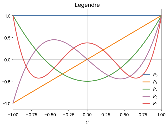
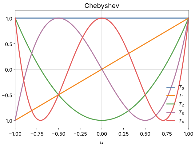
Legendre and Chebyshev span the same function space; which fits a given dataset better is an empirical question, and on smooth data they often perform similarly.

The squash

The polynomials are bounded only on \([-1, 1]\); outside it they grow like \(u^d\). Every input therefore passes through a squash first, chosen by model.squash_method or per entry.

sigma (the default) standardizes the input with its mean and standard deviation, maps the band within squash_n_sigma standard deviations linearly onto \(\pm\)squash_core_range, and saturates smoothly beyond it, never reaching \(\pm 1\). With the defaults (2 and 0.75):

Standard deviations from the mean	Squashed value
0	0
1	0.375
2	0.75 (edge of the linear band)
3	0.936
4	0.973
5	0.985
10	0.997

The bulk of the data passes through undistorted, and outliers keep their order without leaving \((-1, 1)\). The mean and standard deviation are those of the layer's actual inputs, measured on the train split in one pass before the layer trains (Trainer.fit_layer_inputs), separately for every input of every candidate.

tanh needs no statistics, but it compresses the bulk: it is already at 0.762 one standard deviation out.

squash: false feeds the inputs unchanged, for inputs already inside \([-1, 1]\).

Because the squash bounds the basis inputs, it mainly improves conditioning: it tends to tighten the run-to-run spread and speed up the per-neuron fits, usually with little effect on the central accuracy.

Options

Option	Default	Meaning
degree	3	highest polynomial degree per input
dim	2	inputs per neuron
cross	true	include the pairwise products \(u_k u_l\)
squash	true	squash the inputs into \((-1, 1)\)
squash_method	model.squash_method (sigma)	sigma or tanh
squash_n_sigma	model.squash_n_sigma (2.0)	half-width of the linear band, in standard deviations
squash_core_range	model.squash_core_range (0.75)	squashed value at the band's edge, in \((0, 1)\)
activation	identity	output activation

model:
  ref_functions:
    - legendre:
        degree: 3
    - legendre:
        degree: 3
        dim: 4

Raising degree past 3 adds higher-order curvature but often brings little on smooth data. Raising dim lets a single neuron model joint interactions across more than two inputs, which the pairwise families reach only indirectly; whether it helps depends on how much of the signal lives in those interactions.

In logs and plots

The short name joins the basis and the degree, with the number of inputs when it is not 2: Legendre3, Chebyshev4, Legendre3x4.

The knobs

model.ref_functions with the options above, model.squash_method, model.squash_n_sigma and model.squash_core_range. See Configuration keys.

Checked against TorchSONN 0.1.5.