Power-basis polynomials

The power-basis families build their design rows from plain powers and products of their inputs. They are the partial descriptions of classical GMDH (see the Kolmogorov-Gabor polynomial).

The pair families

linear, linear_cov, quadratic and cubic read two inputs \(x_i\) and \(x_j\):

Family	Neuron	Weights
linear	\(w_0 + w_1 x_i + w_2 x_j\)	3
linear_cov	\(w_0 + w_1 x_i + w_2 x_j + w_3 x_i x_j\)	4
quadratic	\(w_0 + w_1 x_i + w_2 x_j + w_3 x_i^2 + w_4 x_j^2 + w_5 x_i x_j\)	6
cubic	the quadratic terms \(+\ w_6 x_i^3 + w_7 x_j^3\)	8

quadratic holds every term up to degree 2. cubic adds the pure cubes but not the mixed terms \(x_i^2 x_j\) and \(x_i x_j^2\). These families take no options besides activation.

polyquad: more than two inputs

polyquad is a degree-2 polynomial over dim inputs:

\[ y = w_0 + \sum_{k} w_k x_k + \sum_{k \le l} w_{kl}\, x_k x_l \]

with 1 + dim + dim(dim+1)/2 weights: 21 at dim: 5. With squares: false, the squares \(x_k^2\) are left out and only the cross products remain, which saves dim weights.

Option	Default	Meaning
dim	2	inputs per neuron
squares	true	include the squared terms
activation	identity	output activation

model:
  ref_functions:
    - polyquad:
        dim: 5
        squares: true

A layer with \(n\) inputs has \(\binom{n}{\text{dim}}\) tuples, which grows fast with dim: 16 inputs make 4,368 tuples of 5. model.max_neuron_models caps how many a layer tries. With a dim above 2, polyquad needs that cap: it cannot enumerate its tuples, and without the cap building the first layer raises NotImplementedError.

Conditioning and heavy tails

The power basis has a weakness that grows with the degree. Over a fixed range, the powers \(x, x^2, x^3, \dots\) look more and more alike as the degree rises (odd powers resemble each other, and so do even ones), so their columns become nearly collinear and the least-squares problem for their weights becomes poorly conditioned. Heavy-tailed inputs make it worse: a feature 10 standard deviations out contributes \(10^3\) to a cube term, and those few rows dominate the fit. The power-basis families use their inputs as they come, so this falls on the data preparation: standardize, and clip or transform the far tails (see the regression quickstart).

Both effects show up in the powers themselves. Near the origin the curves bunch together, so their columns carry almost the same information; away from it the high powers climb steeply, so a single far-out row can swamp the rest.

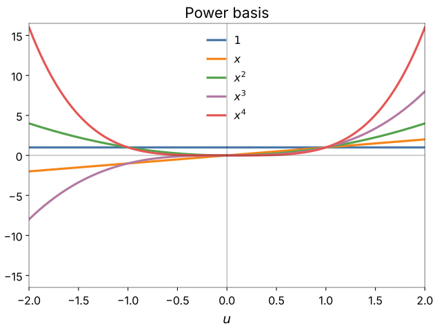
The higher-degree families (quadratic, cubic) feel this most: the extra terms they add are the ill-conditioned ones, so they can be less stable across runs without being more accurate. The orthogonal families avoid the problem by squashing each input into \([-1, 1]\) and using a basis that stays well conditioned there.

In logs and plots

The short names are Linear, LinearCov, Quadratic, Cubic and poly<dim>, for example poly5.

The knobs

model.ref_functions with the options above, and model.max_neuron_models. See Configuration keys.

Checked against TorchSONN 0.1.5.