TorchSONN
TorchSONN is a PyTorch library for building and training self-organizing deep neural networks. The network grows one layer at a time. Each layer builds candidate neurons, small functions of two or more inputs taken from the previous layers' outputs and the original features. Every candidate is fitted on the training split, and the ones with the lowest error on a held-out split (by default, a separate dev split) survive into the next layer. The search stops when adding layers stops lowering that error.
The neurons come from three families: plain polynomials, orthogonal polynomials and Gaussian radial basis functions. Once the network has grown, it can be refined: a linear output head combines the last layer's survivors, and an end-to-end pass trains every parameter of the network at once by gradient descent.
The result is a network you can read: every neuron is an explicit formula over a few named inputs, and the whole network can be drawn as a graph.
Neuron families
- Plain polynomials in the power
basis:
linear,linear_cov,quadratic,cubicand the multi-inputpolyquad. - Orthogonal polynomials:
legendreandchebyshev, with a configurable degree and number of inputs. They stay well conditioned at higher degrees, where the raw power basis does not. - Gaussian radial basis functions:
rbf, local bumps whose centres and widths start from k-means and are then learned.
How a model grows
flowchart LR
    F[Features] --> L0[Layer 0]
    L0 --> L1[Layer 1]
    F --> L1
    L1 --> L2[...]
    F --> L2
    L2 --> P[Prediction]
Each layer fits its candidates on the train split and keeps the
nbest_neurons with the lowest dev error. Growth stops when the dev error
stops improving, and the model keeps the layers up to the best one. The
prediction is read off the grown network in one of two ways:
- Best neuron (default): the single last-layer survivor with the lowest dev error becomes the output. This is the classic GMDH read-out, and it keeps the model reducible to one explicit formula.
- Linear head: with
use_output_projection, a linear layer combines several of the last layer's survivors into the prediction, which an end-to-end pass can then refine by training every parameter at once. This usually fits better, at the cost of the single-formula reading.
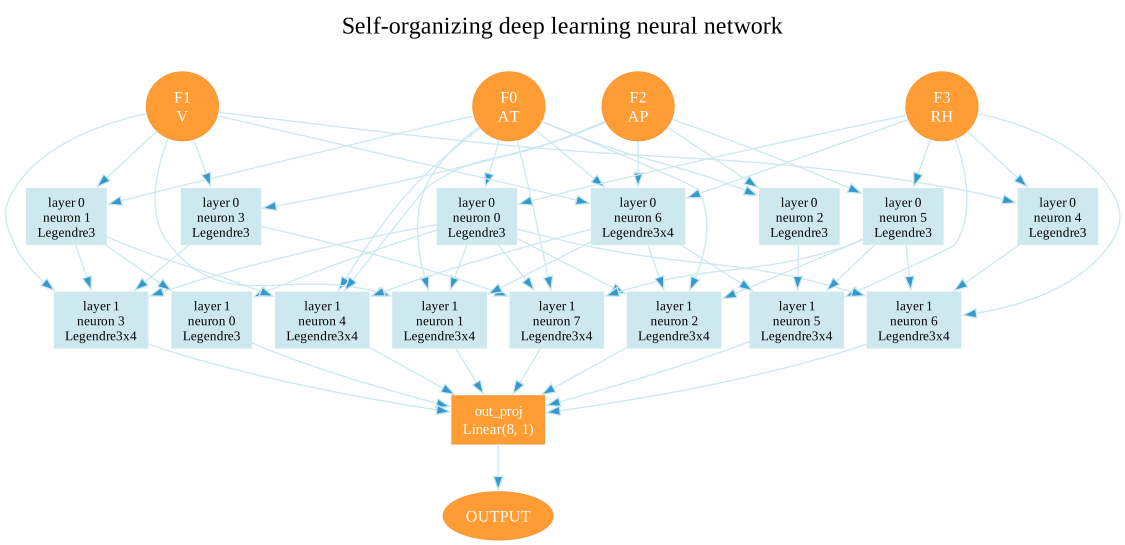
A grown network
The network of the CCPP tutorial, pruned to the
neurons that reach the output. Each box is a neuron, and its incoming edges
are the inputs it reads. PlotModel draws it (see
Inspecting a model); click the image for full size.
Relation to GMDH
TorchSONN builds on the Group Method of Data Handling (GMDH) and on GmdhPy, a scikit-learn-style GMDH library. Two parts come from GMDH: the plain-polynomial neurons, and the growth itself, which fits candidates layer by layer and keeps the best by their error on a separate split. The orthogonal-polynomial and RBF neurons, the output head, the fine-tuning passes and the training on a GPU go beyond it. GMDH describes the method.
Example
California housing regression on the CPU:
import numpy as np
from omegaconf import OmegaConf
from sklearn.datasets import fetch_california_housing
from sklearn.preprocessing import StandardScaler
from torch.utils.data import DataLoader
from torchsonn import SONN, SONNDataset, Trainer

# The rows come grouped by location, so shuffle before splitting:
# 50% train, 25% dev, 25% test; standardize on the train rows only.
x, y = fetch_california_housing(return_X_y=True)
order = np.random.default_rng(0).permutation(len(x))
x, y = x[order], y[order]
i_train, i_dev = int(0.50 * len(x)), int(0.75 * len(x))
x = StandardScaler().fit(x[:i_train]).transform(x).astype(np.float32)
# A few rows sit hundreds of standard deviations out (population, average
# occupancy); clip them so the polynomials do not extrapolate there.
x = np.clip(x, -5.0, 5.0)
y = y.astype(np.float32)

def loader(start, stop, shuffle=False):
    dataset = SONNDataset(x[start:stop], y[start:stop])
    # One batch holds a whole split (10,320 training rows).
    return DataLoader(dataset, batch_size=16384, shuffle=shuffle)

train_dl = loader(0, i_train, shuffle=True)
dev_dl = loader(i_train, i_dev)
test_dl = loader(i_dev, None)

# Only what differs from the defaults in torchsonn.config.SONNConfig.
config = OmegaConf.merge(SONN.default_config(), {
    "model": {
        "type": "regressor",
        "ref_functions": ["linear_cov"],
        "nbest_neurons": 8,
        "max_neuron_models": 28,
    },
    "train": {
        "max_layer_count": 10,
        "steps": 500,
        "eval_step_interval": 5,
        "early_stop_patience": 1e-4,
        "early_stop_tolerance_steps": 3,
        "checkpoint_dir": "checkpoints/california",
        "optimizer": {
            "name": "lbfgs",
            "optimizer_params": {
                "lr": 0.1, "min_lr": 0.01, "history_size": 10,
            },
        },
    },
})

Trainer.set_seed(config.train.seed)
model, trainer = SONN(config, d_model=x.shape[1]), Trainer(config)
trainer.train(model, train_dl, dev_dl, test_dl)
trainer.load_model_checkpoint(model, "cpu")
preds, targets = trainer.infer(model, test_dl)
print(f"test MSE: {((preds - targets) ** 2).mean().item():.4f}")
Where next
- To fit a model: install the package, work through a quickstart for regression or classification, then use the guides and the configuration keys.
- If you know GMDH or polynomial networks: start with GMDH, the Kolmogorov-Gabor polynomial and the algorithm, then the criteria and stopping rules with the exact formulas the code uses.
- To work on the code: the API reference.